Building your first data flow

Before querying data, make sure you have installed the latest Ananas Analytics Desktop first.

In this tutorial we will build our first data flow with Ananas Analtyics Desktop, to analyze the 2019 FIFA football players dataset, which can be downloaded from fifa2019.csv

You can download Ananas Desktop Examples, and import them to Ananas Desktop for quick start.

Create a project

Ananas Analytics Desktop lets you organize your analysis work by projects. Ananas project consists of an analysis board where a set of steps can be connected to each other.

To create your first project, click on the + button then fill in the project name and description.

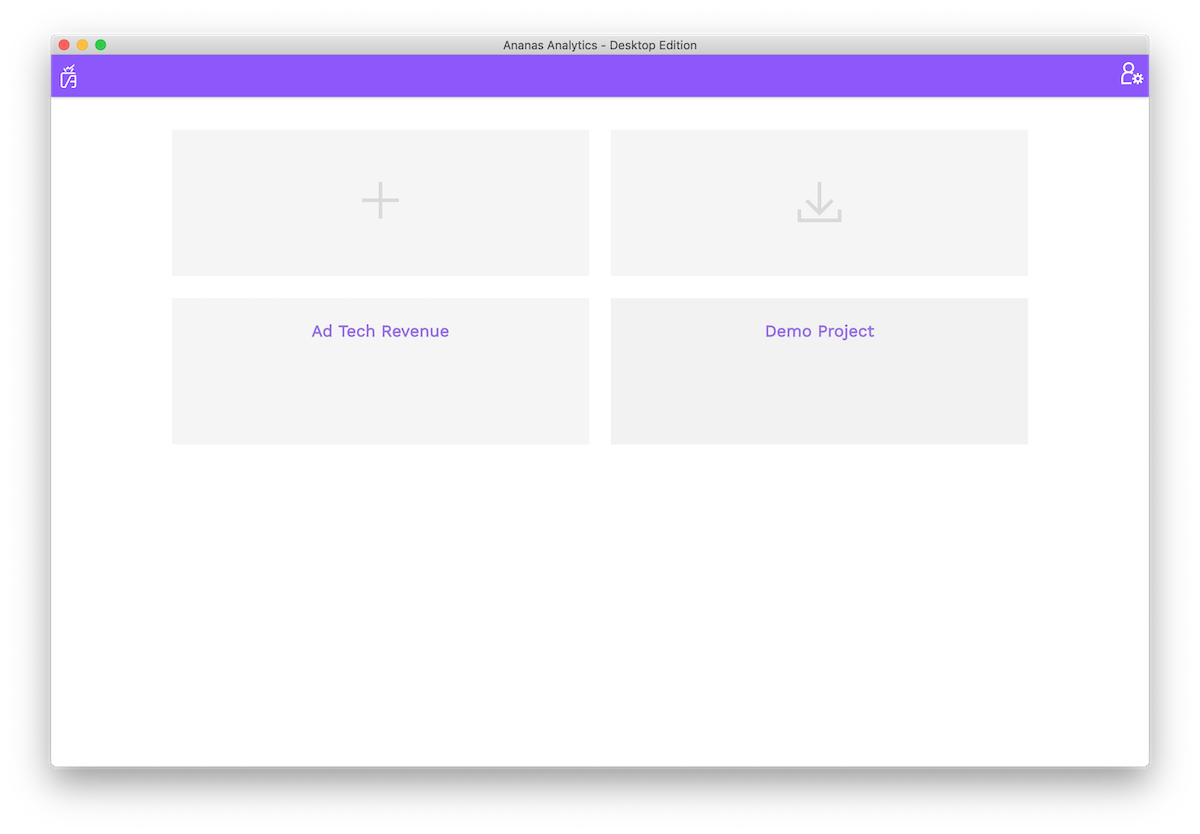
Now you've created your first project. You can start working on your project analysis board.

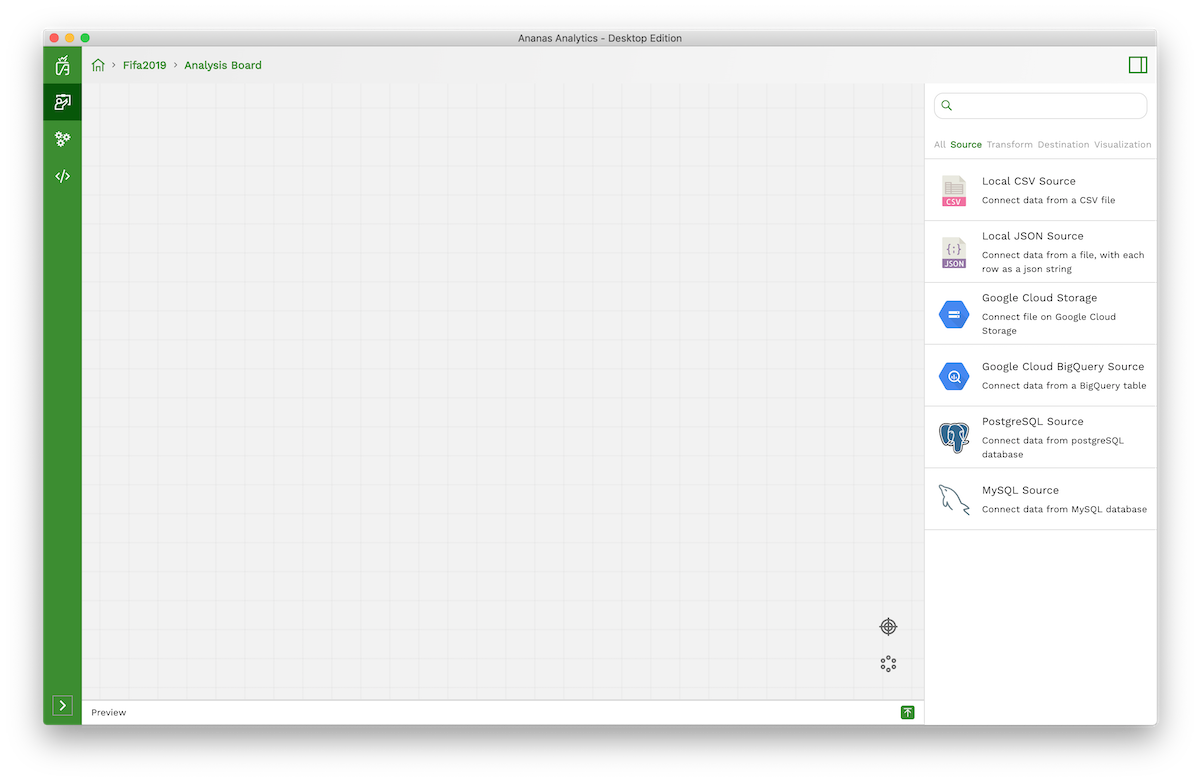
Connect & configure data source

Any analysis begins with a data source. For our get started project, we can drag & drop Local CSV Source from the right side tool box to your analysis board.

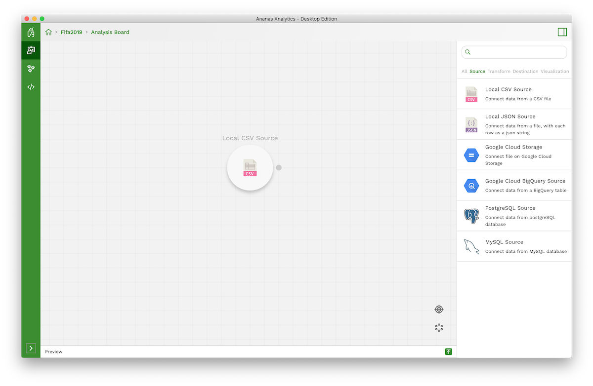
Click the newly created Local CSV Source step, and click the settings action (first action displays under the step) to start configure the data source.

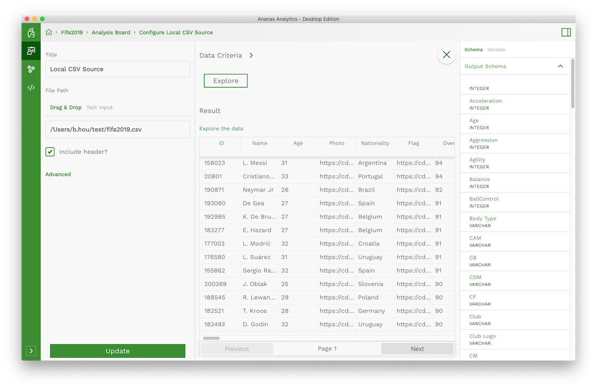
Drag & drop the downloaded fifa2019.csv file to the File Path settings. Click Explore to view the data source.

In Ananas Analytics, we encourage the fail-fast testing best practise for each step. The Explore button provides not only the capability to explore the data source, but also two additional important functionalities:

• Test the current step settings
• Auto-detect the data schema (the data columns and their types) and display it on the right side contextual toolbox

Analysis (transform)

Now we have explored our dataset, it's time to do some analysis! In Ananas Analytics, an analysis is constructed by multiple transforms. The most useful transform is SQL transform, which provides you the possibility to analyze(transform) your dataset with standard SQL.

Drag & drop an SQL transform to your analysis board, and connect the created fifa2019 csv source to it.

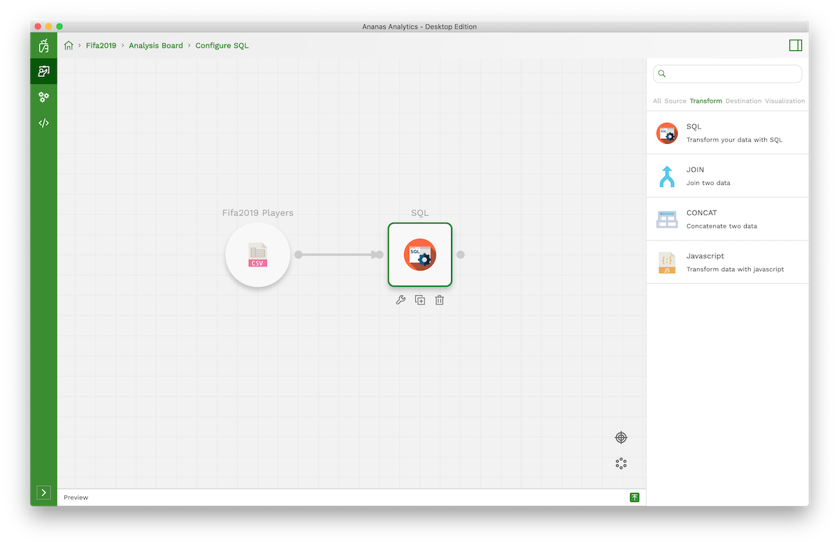
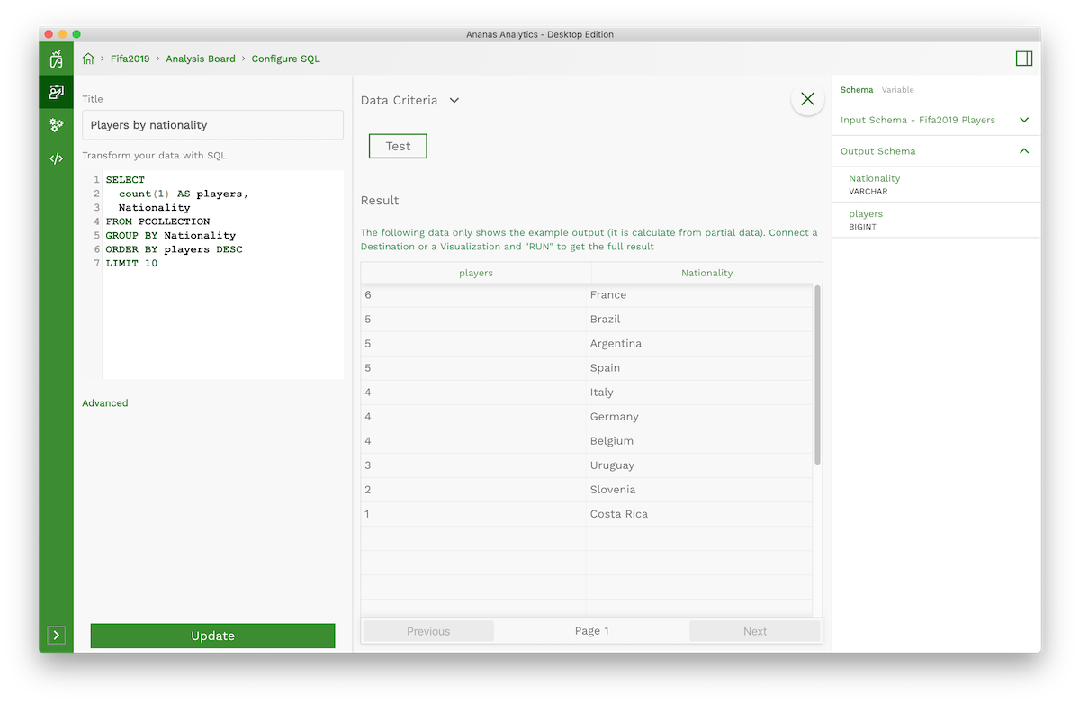
Open the SQL transform settings editor, type the following SQL:

SELECT 
    count(1) AS players,
    Nationality
FROM PCOLLECTION
GROUP BY Nationality
ORDER BY players DESC
LIMIT 10

The above simple SQL counts the top 10 nationalities.

Before we move to next step, we need to test the current settings by clicking the Test button. In a few seconds, it will display the test result and the auto-detected output schema.

The test result is not the final query result. Under the hood, Ananas Analytics takes a few sample data from your dataset and then runs the step to test the current settings. What's more, it auto-detects the output data schema. The fail-fast testing makes it possible to test big data set (for example, Terabytes data) in seconds.

Run & Visualize the result

Until now, we have tested our analysis settings in one minute. To get the final result, we need to store the result to a destination (for example, a file, a database), or a visualization.

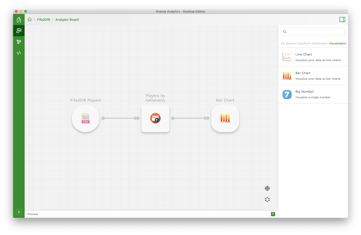
Drag & drop a Bar chart Visualization step to analysis board, and connect it from the SQL transform

Open the Bar chart settings editor, config the dimensions, measures, chart title, X axis label, Y axis label, and then click Test to test your settings in seconds.

Once you passes the test, click the RUN button to submit a job to execute the analysis in background. You will get a system notification when the job is DONE or FAILED.

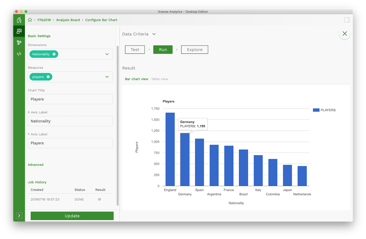
Once the job is DONE, you can click the Explore button (or the eye icon from the job in job history) to view the final result in the bar chart editor.

Congratulations! You just made your first analysis with Ananas Analytics Desktop.